Prior elicitation

Test case

set.seed(1337)

library(bayessource)
requireNamespace("mvtnorm")
#> Loading required namespace: mvtnorm

Let’s generate a test dataset with known parameters.
We will use some supporting functions:

# Generate n random integers in {min, ..., max}
randi <- function(n, min, max) {
   round(runif(n, min, max))
}

#' Generate random invertible symmetric pxp matrix
#'
#' @param p matrix size
#' @param alpha regularization > 0
randinvmat <- function(p, M = 5, alpha = NULL) {
   stopifnot(p > 0)
   stopifnot(M > 0)
   if (is.null(alpha)) {
      alpha <- p + 1
   } else {
      stopifnot(alpha > 0)
   }
   M * stats::rWishart(1, p + alpha, diag(p))[, , 1] / (p + alpha)
}

# Compute inverse of X if X is symmetric-positive definite
solve_sympd <- function(X) {
   chol2inv(chol(X))
}

Data generation

We will generate the data according to the model: for sources \(i = 1, \ldots, m\),

\[\begin{align} X_{ij} \mid \theta_i, \; W_i &\sim N_p(\theta_i, W_i) \quad \forall j = 1, \ldots, n \\ \theta_i \mid \mu, B &\sim N_p(\mu, B) \\ W_i \mid U, n_w &\sim IW(U, n_w) \end{align}\]

p <- 4 # number of variables
m <- 100 # number of sources
n <- 500 # number of items per source

Upper hierarchical level: choose some generating hyperparameters \(\mu\), \(n_w\), \(B\), \(U\)

list_exact <- list()
list_exact$B.exact <- randinvmat(p, alpha = 2) # Between Covariance matrix
list_exact$U.exact <- randinvmat(p, alpha = 2) # Inverted Wishart scale matrix
list_exact$mu.exact <- randi(p, 0, 10) # mean of means
list_exact$nw.exact <- 2 * (p + 1) + 1 # dof for Inverted Wishart, as small as possible

Middle hierarchical level: for each \(i\)-th source generate

true source mean: \(\theta_i\)
true within-source covariance matrix: \(W_i\)

theta.sources.exact <- list()

for (i in seq(m)) {
   theta.sources.exact[[i]] <- mvtnorm::rmvnorm(1, list_exact$mu.exact, list_exact$B.exact)
}

# Sample from an inverted Wishart
W.sources.exact <- list()
for (i in seq(m)) {
   # ours:
   W.sources.exact[[i]] <- bayessource::riwish_Press(list_exact$nw.exact, list_exact$U.exact)
   # R:
   # W.sources.exact[[i]] <- solve(rWishart(1, nw.exact, solve(U.exact))[,,1])
}

Lower hierarchical level: generate raw data from every source

df <- list()
for (i in seq(m)) {
   # Sample data from the i-th source
   # returned as a matrix
   df[[i]] <- mvtnorm::rmvnorm(n, theta.sources.exact[[i]], W.sources.exact[[i]])
   # Store the true source in the last column
   df[[i]] <- cbind(df[[i]], i)
}

# Convert to a dataframe
# columns v_1, v_2, ..., v_p, source
df <- data.frame(do.call(rbind, df))
colnames(df) <- paste(c(paste0("v", seq(1:p)), "source"))

head(df)
#>         v1        v2         v3       v4 source
#> 1 7.783807 2.3526976  1.1456413 3.235036      1
#> 2 7.478913 4.1146210  0.8399942 1.533766      1
#> 3 7.490046 3.7630065  0.6714497 1.734876      1
#> 4 7.228848 0.7886417 -0.5594819 3.323668      1
#> 5 7.354987 1.7059334  1.9262933 2.380303      1
#> 6 6.920879 2.4161567  3.0941613 1.858068      1

The item column is the last one (p + 1).

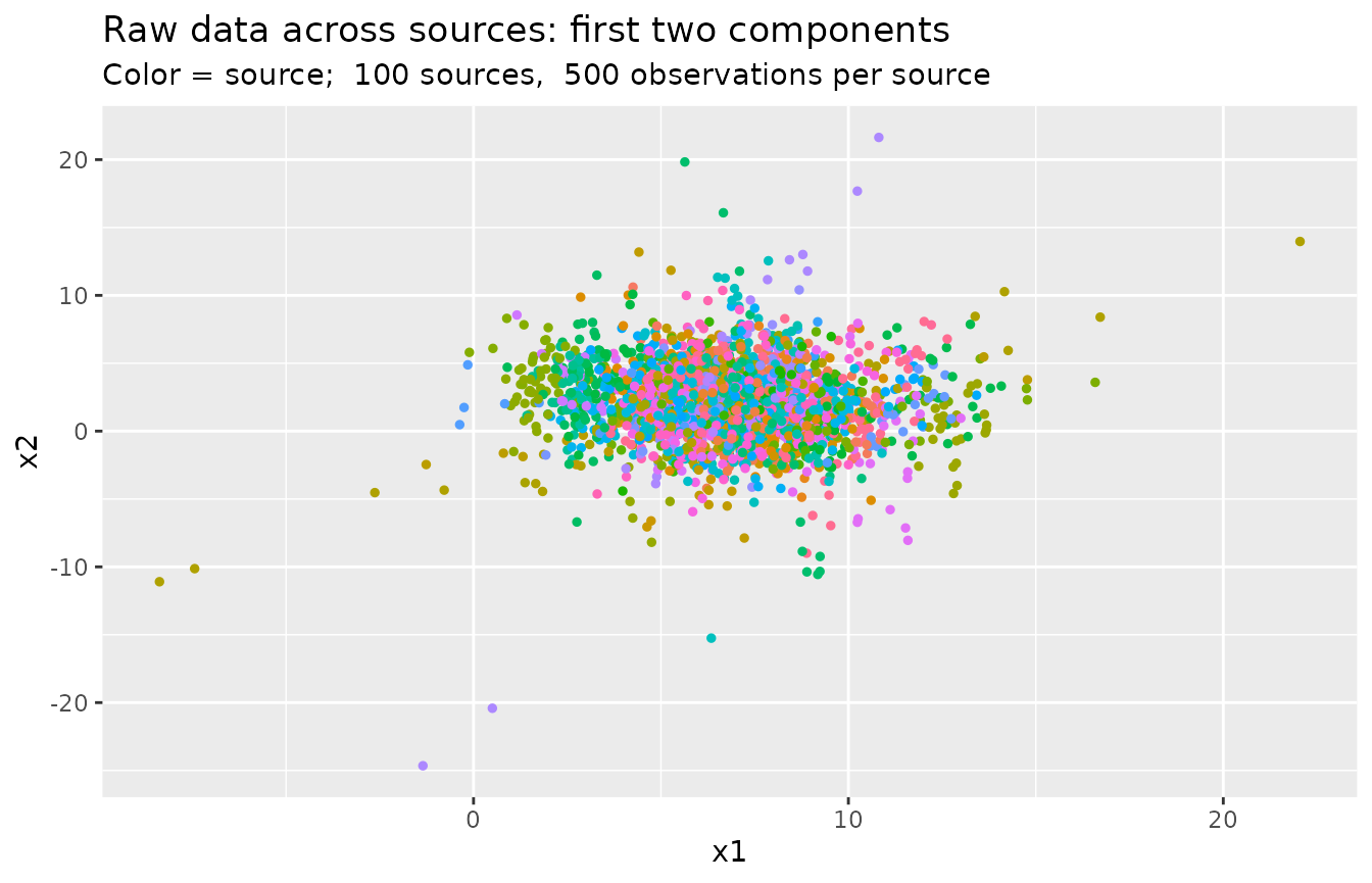
Visualization

Show the first two components across sources:

library(ggplot2)

df_sub <- df[sample(1:nrow(df), nrow(df) * 0.05, replace = FALSE), ]

ggplot(df_sub, aes(x = v1, y = v2, col = factor(source))) +
   geom_point(size = 1, show.legend = FALSE) +
   labs(
      x = "x1",
      y = "x2",
      title = "Raw data across sources: first two components",
      subtitle = paste("Color = source; ", m, "sources, ", n, "observations per source")
   )

The package supplies the function make_priors_and_init().

Suppose that df represents a background dataset.
We can use it to elicit the model hyperparameters using the estimators described in [@Bozza2008Probabilistic].
It also chooses an initialization value for the Gibbs sampler.

col.variables <- 1:p
col.item <- p + 1

use.priors <- "ML"
use.init <- "random"

priors <- make_priors_and_init(df, col.variables, col.item, use.priors, use.init)
names(priors)
#> [1] "mu"      "U"       "B.inv"   "nw"      "W.inv.1" "W.inv.2"

Hyperpriors on mean

\[\theta_i \mid \mu, B \sim N_p(\mu, B)\]

Hyperprior for the between-sources mean \(\mu\):

## priors$mu

\[ \hat{'mu} = \begin{bmatrix} 6.8288 \\ 2.0473 \\ 0.8846 \\ 2.9926 \\ \end{bmatrix} \]

Exact:

## list_exact$mu.exact

\[ \mu = \begin{bmatrix} 7.0000 \\ 2.0000 \\ 1.0000 \\ 3.0000 \\ \end{bmatrix} \]

Hyperprior for the between-sources covariance matrix \(B\):

## priors$B.inv

\[ \hat{B}^{-1} = \begin{bmatrix} 1.1238 & 0.9870 & -0.7478 & -0.0710 \\ 0.9870 & 2.1015 & -0.8342 & 0.1850 \\ -0.7478 & -0.8342 & 0.8177 & -0.1066 \\ -0.0710 & 0.1850 & -0.1066 & 0.1953 \\ \end{bmatrix} \]

Exact:

## list_exact$B.exact

\[ B^{-1} = \begin{bmatrix} 0.9970 & 0.9335 & -0.7219 & 0.0117 \\ 0.9335 & 2.0978 & -0.7957 & 0.1698 \\ -0.7219 & -0.7957 & 0.7742 & -0.1125 \\ 0.0117 & 0.1698 & -0.1125 & 0.1440 \\ \end{bmatrix} \]

Hyperpriors on within covariance matrix

\[ W_i \sim IW(n_w, U) \]

Inverted Wishart degrees of freedom: arbitrary, chosen as low as possible (largest variance) s.t. the expected value of \(W_i\) is defined

\[n_w = 11\]

Inverted Wishart scale matrix:

## priors$U

\[ \hat{U} = \begin{bmatrix} 1.6633 & 1.1123 & -1.3456 & 1.6272 \\ 1.1123 & 8.8548 & -1.6904 & -0.6213 \\ -1.3456 & -1.6904 & 13.1649 & 2.2322 \\ 1.6272 & -0.6213 & 2.2322 & 5.0199 \\ \end{bmatrix} \]

Exact:

## list_exact$U.exact

\[ U = \begin{bmatrix} 0.9172 & 1.1136 & -1.1124 & 0.5796 \\ 1.1136 & 11.4074 & -3.4977 & -1.5801 \\ -1.1124 & -3.4977 & 12.3324 & 2.6193 \\ 0.5796 & -1.5801 & 2.6193 & 3.9750 \\ \end{bmatrix} \]

Initialisation

Within-source covariance matrices and their inverses: we initialize the chain with

## priors$W.inv.1
## priors$W.inv.2

\[ W^{-1}_1 = \begin{bmatrix} 8.2080 & -1.2025 & 0.2300 & -5.1136 \\ -1.2025 & 0.6395 & 0.1093 & 0.6541 \\ 0.2300 & 0.1093 & 0.7650 & -1.1145 \\ -5.1136 & 0.6541 & -1.1145 & 4.6794 \\ \end{bmatrix} \]\[ W^{-1}_2 = \begin{bmatrix} 8.2080 & -1.2025 & 0.2300 & -5.1136 \\ -1.2025 & 0.6395 & 0.1093 & 0.6541 \\ 0.2300 & 0.1093 & 0.7650 & -1.1145 \\ -5.1136 & 0.6541 & -1.1145 & 4.6794 \\ \end{bmatrix} \]

Usage

The list returned by make_priors_and_init() can be used in calls to marginalLikelihood() and samesource_C():

priors <- make_priors_and_init(df, col.variables, col.item, use.priors, use.init)

mtx_data <- as.matrix(df[, col.variables])

ml <- marginalLikelihood(
   X = mtx_data,
   n.iter = 1000,
   burn.in = 100,
   B.inv = priors$B.inv,
   W.inv = priors$W.inv.1,
   U = priors$U,
   nw = priors$nw,
   mu = priors$mu
)

ml
#> [1] -509497.2

bf <- samesource_C(
   quest = mtx_data,
   ref = mtx_data,
   n.iter = 1000,
   burn.in = 100,
   B.inv = priors$B.inv,
   W.inv.1 = priors$W.inv.1,
   W.inv.2 = priors$W.inv.1,
   U = priors$U,
   nw = priors$nw,
   mu = priors$mu
)

bf
#> [1] 80.74815

Prior elicitation

Lorenzo Gaborini

2021-11-05

Test case

Data generation

Visualization