Dirichlet distribution tools

This package contains functions to sample from a Dirichlet distribution.

Notation

We call \(\text{Simplex}{(p-1)}\) the set of vectors in \(\mathbb{R}^p\) whose components form a distribution on \(p\) items.
In other words, \(\boldsymbol{X} \in \text{Simplex}{(p-1)}\) iff \(X_i \in [0,1]\) and \(\sum_{i=1}^p X_i = 1\).

Let \(\boldsymbol{X}\) be a vector in \(\text{Simplex}{(p-1)}\), let \(\boldsymbol{\alpha}\) be a vector in \(\mathbb{R}^p\) with positive components.

Then, \(X\) can have the Dirichlet distribution: \(X \mid \boldsymbol{\alpha} \sim \text{Dirichlet}{(\boldsymbol{\alpha})}\).

We can write \(\boldsymbol{\alpha} = \alpha_0 \, \boldsymbol{\nu}\), where:

\(\alpha_0 = \sum_i \alpha_i\) is the concentration parameter: \(\alpha_0 \in \mathbb{R}^{+}\)
\(\boldsymbol{\nu}\) is the base measure: \(\boldsymbol{\nu} \in \text{Simplex}{(p-1)}\).

Properties

\(\mathop{\mathbb{E}}[\boldsymbol{X}] = \boldsymbol{\alpha} / \alpha_0 = \boldsymbol{\nu}\)
\(\mathop{\mathrm{Var}}[\boldsymbol{X}] = \dfrac{ \boldsymbol{\nu} \cdot (1 - \boldsymbol{\nu})}{\alpha_0 + 1}\)

Particular cases

If \(\boldsymbol{\nu}\) is constant, \(\boldsymbol{\nu} = 1/p\). The Dirichlet distribution is called symmetric Dirichlet, and is only parametrised by the concentration parameter \(\alpha_0\).

When \(\alpha_0 = p\), \(\alpha_i = 1 \forall i\): the Dirichlet distribution is uniform over \(\text{Simplex}{(p-1)}\). This is the least informative situation.
When \(\alpha_0 \to 0\), \(\alpha_i \to 0\): the Dirichlet distribution concentrates over the border of \(\text{Simplex}{(p-1)}\).
When \(\alpha_0 \gg 1\), \(\alpha_i \to 0\): the Dirichlet distribution concentrates over the mean (and the variance decreases).

Examples

Sample from a \(p=4\) Dirichlet:

n <- 100

# The parameter
alpha <- c(0.5, 0.1, 5, 0.1)
p <- length(alpha)

# Concentration and base measure
alpha0 <- sum(alpha)
nu <- alpha / alpha0

\(\alpha_0 = 5.7\)
\(\boldsymbol{\nu} = \left( 0.0877193, 0.0175439, 0.877193, 0.0175439 \right)\)
\(\boldsymbol{\alpha} = \left( 0.5, 0.1, 5, 0.1 \right)\)

df_diri <- fun_rdirichlet(n, alpha)
head(df_diri)
#> # A tibble: 6 x 4
#>     `x[1]`   `x[2]` `x[3]`   `x[4]`
#>      <dbl>    <dbl>  <dbl>    <dbl>
#> 1 0.0243   9.74e- 4  0.901 7.33e- 2
#> 2 0.0465   4.45e- 7  0.902 5.17e- 2
#> 3 0.0625   3.00e- 3  0.890 4.47e- 2
#> 4 0.158    1.07e- 4  0.842 4.17e- 7
#> 5 0.000115 5.70e-20  1.00  1.10e-19
#> 6 0.397    1.44e- 6  0.603 8.62e-11

#> Loading required namespace: GGally
#> Registered S3 method overwritten by 'GGally':
#>   method from   
#>   +.gg   ggplot2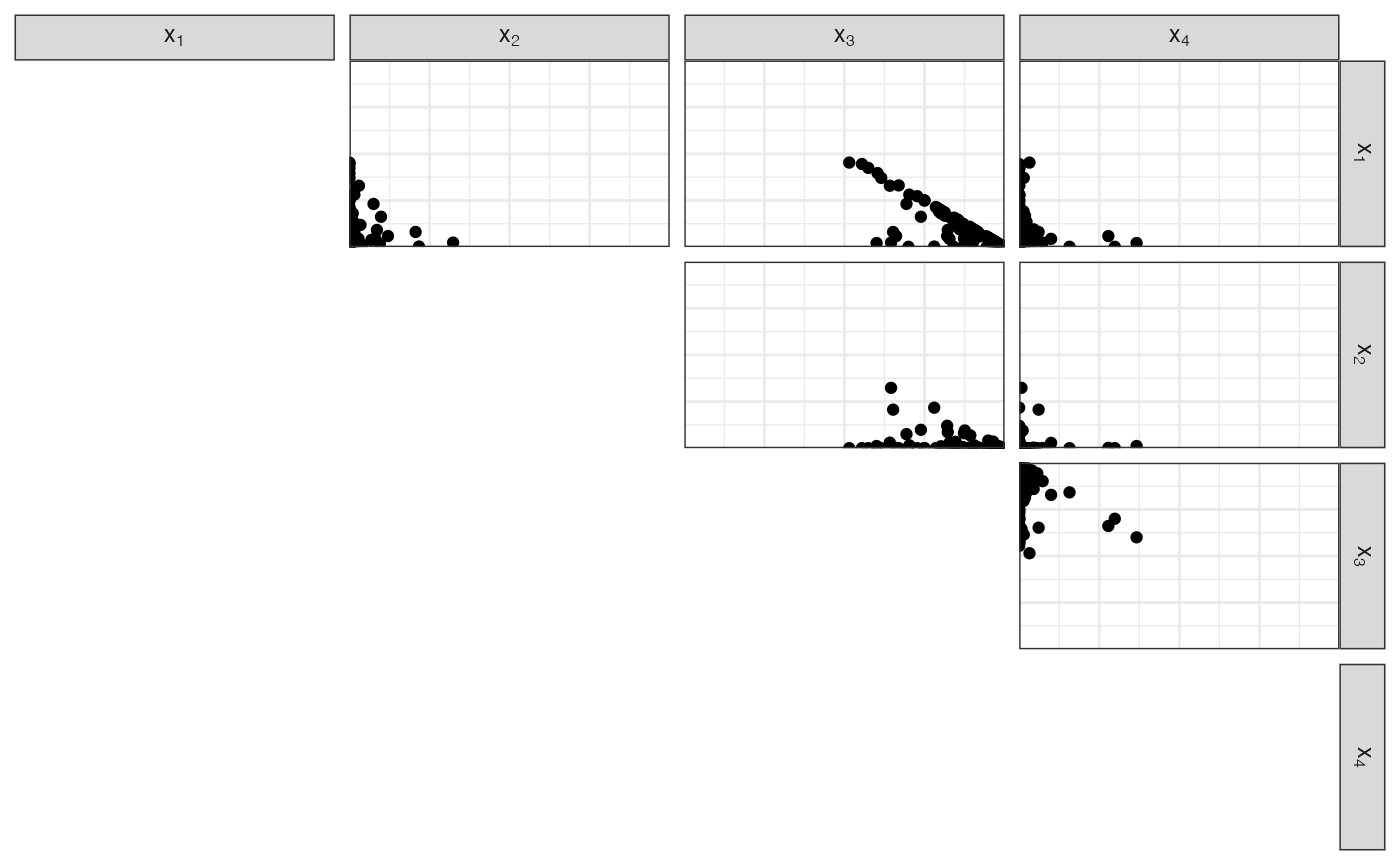

Uniform sampling

Uniform base measure, unitary Dirichlet parameters: \(\boldsymbol{\alpha} = \boldsymbol{1}\).

nu <- rep(1, p)/p
alpha0 <- p
alpha <- nu * alpha0

\(\alpha_0 = 4\)
\(\boldsymbol{\nu} = \left( 0.25, 0.25, 0.25, 0.25 \right)\)
\(\boldsymbol{\alpha} = \left( 1, 1, 1, 1 \right)\)

df_diri <- fun_rdirichlet(n, alpha)
head(df_diri)
#> # A tibble: 6 x 4
#>   `x[1]` `x[2]` `x[3]` `x[4]`
#>    <dbl>  <dbl>  <dbl>  <dbl>
#> 1 0.0269 0.289  0.529  0.155 
#> 2 0.117  0.0997 0.158  0.625 
#> 3 0.302  0.372  0.133  0.194 
#> 4 0.549  0.260  0.0809 0.110 
#> 5 0.139  0.493  0.0720 0.297 
#> 6 0.223  0.244  0.485  0.0483

scatter_matrix_simplex(df_diri)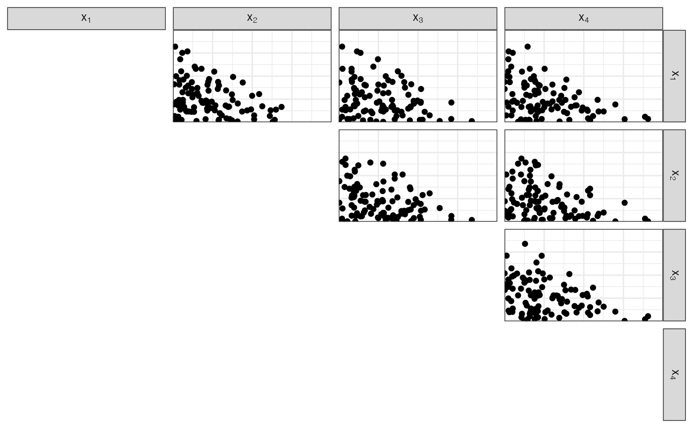

Concentrated sampling

Concentration parameter \(\gg p\), Dirichlet parameters \(\gg 1\)

nu <- rep(1, p)/p
alpha0 <- 100
alpha <- nu * alpha0

\(\alpha_0 = 100\)
\(\boldsymbol{\nu} = \left( 0.25, 0.25, 0.25, 0.25 \right)\)
\(\boldsymbol{\alpha} = \left( 25, 25, 25, 25 \right)\)

df_diri <- fun_rdirichlet(n, alpha)
head(df_diri)
#> # A tibble: 6 x 4
#>   `x[1]` `x[2]` `x[3]` `x[4]`
#>    <dbl>  <dbl>  <dbl>  <dbl>
#> 1  0.257  0.294  0.211  0.239
#> 2  0.202  0.326  0.202  0.269
#> 3  0.199  0.263  0.253  0.284
#> 4  0.241  0.268  0.299  0.192
#> 5  0.281  0.257  0.202  0.259
#> 6  0.220  0.221  0.255  0.304

scatter_matrix_simplex(df_diri)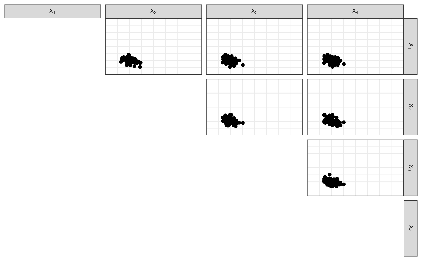

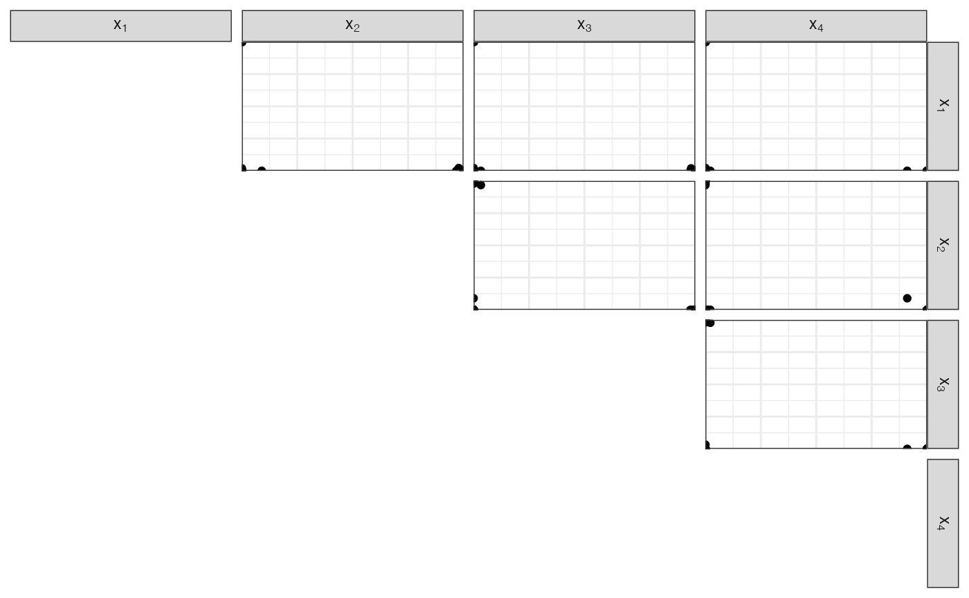
Degenerate sampling

Concentration parameter \(\\ p\), Dirichlet parameters \(\\ 1\)

nu <- rep(1, p)/p
alpha0 <- 0.01
alpha <- nu * alpha0

\(\alpha_0 = 0.01\)
\(\boldsymbol{\nu} = \left( 0.25, 0.25, 0.25, 0.25 \right)\)
\(\boldsymbol{\alpha} = \left( 0.0025, 0.0025, 0.0025, 0.0025 \right)\)

df_diri <- fun_rdirichlet(n, alpha)
head(df_diri)
#> # A tibble: 6 x 4
#>      `x[1]`    `x[2]`   `x[3]`    `x[4]`
#>       <dbl>     <dbl>    <dbl>     <dbl>
#> 1 3.32e-  8 1.00e+  0 5.17e-53 1.92e-139
#> 2 5.03e- 79 6.23e- 46 1.00e+ 0 0.       
#> 3 1.00e+  0 3.22e- 16 3.92e-14 1.41e-154
#> 4 8.03e- 15 9.67e-109 1.00e+ 0 3.43e- 61
#> 5 1.00e+  0 5.86e-103 0.       3.09e- 81
#> 6 1.25e-235 1.18e-182 1.00e+ 0 5.86e-206

scatter_matrix_simplex(df_diri)

Lorenzo Gaborini